Performance Analysis Using Benchmarking Tools

Tools included in Qualcomm Neural Processing SDK

Besides prediction accuracy, two other important aspects of creating a model are low inference time and low memory consumption. Tools in the Qualcomm® Neural Processing SDK™ are designed to help developers and machine learning engineers analyze and improve the performance of the Deep Learning Container (DLC) file.

Consider the example of a pre-trained DLC file used on the preceding pages for facial expression recognition. It achieves acceptable levels of accuracy (68 percent).

DLC Viewer

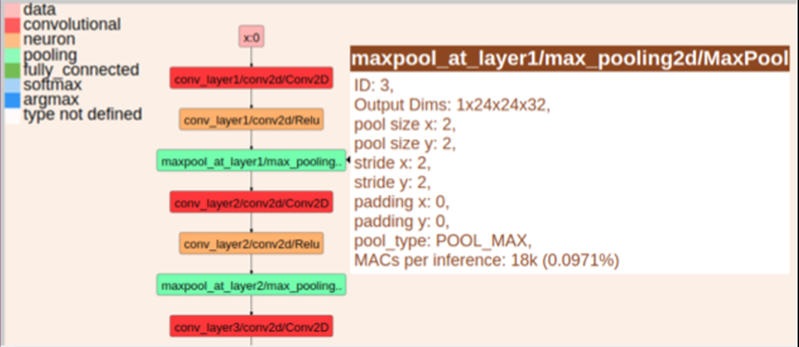
The DLC Viewer tool provided in the SDK allows the engineer to visualize the model and understand its architecture.

The image below illustrates the sample DLC file in DLC Viewer. Moving the cursor over each layer reveals details such as output dimensions, pool size and stride used in the model.

snpe_bench.py

snpe_bench.py is a python script that uses executables and libraries found in the SDK to run a DLC on a target device (Android or embedded Linux). The benchmark collects performance metrics about the neural network, including inference timing and memory consumption.

The input to the benchmark scripts is a configuration file. As a point of departure, the SDK includes a configuration file in JSON format for running the AlexNet model created in the SDK. See Benchmarking in the Qualcomm Neural Processing Engine SDK Reference Guide for a full description and walkthrough, including guidance on creating configuration files ("Create a Run Configuration").

snpe_bench.py works by internally executing snpe-net-run n number of times on a requested runtime over a specified device. A summary is created from the individual "SNPEDiag_0.log",, "SNPEDiag_1.log" ..., "SNPEDiag_n.log" files generated during each execution.

For example, the following command runs the benchmark with fer_model.dlc, configured for 51 iterations on an LG G6 mobile device:

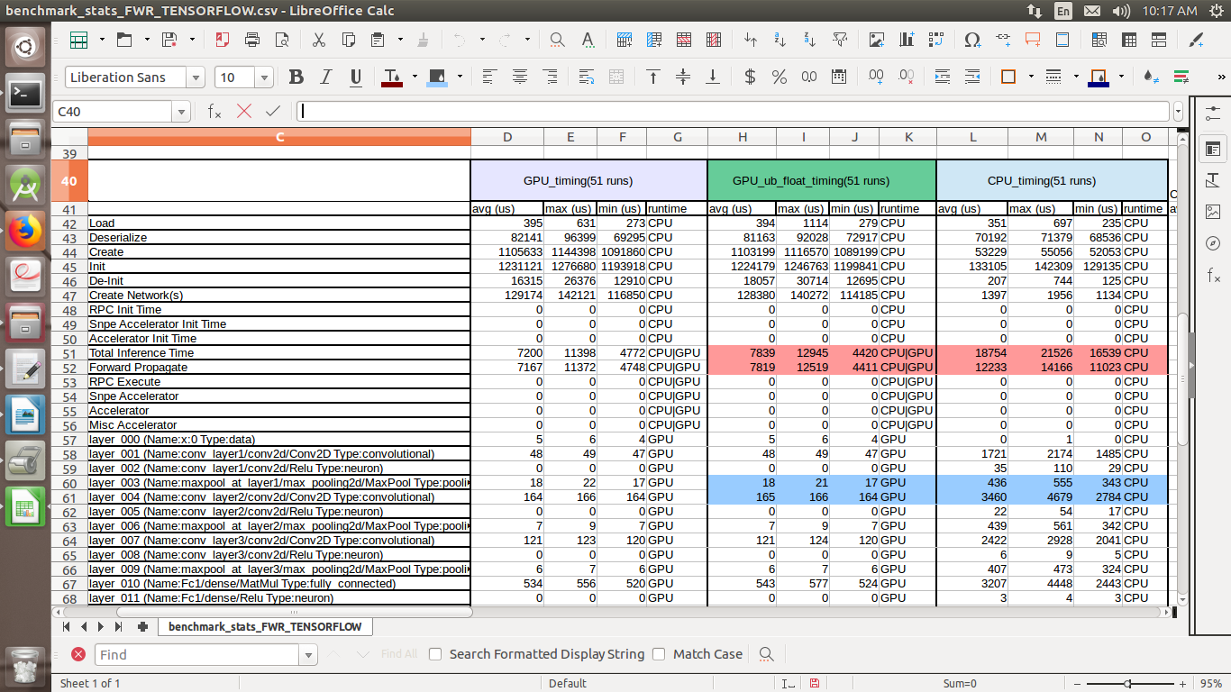
The results are stored as a CSV file, which can also be made available in JSON format. The CSV file contains results similar to the example below. (Note that some measurements may not be apparent in the CSV file. By default, the profiling level is basic; to get all timing information, the profiling level must be detailed.)

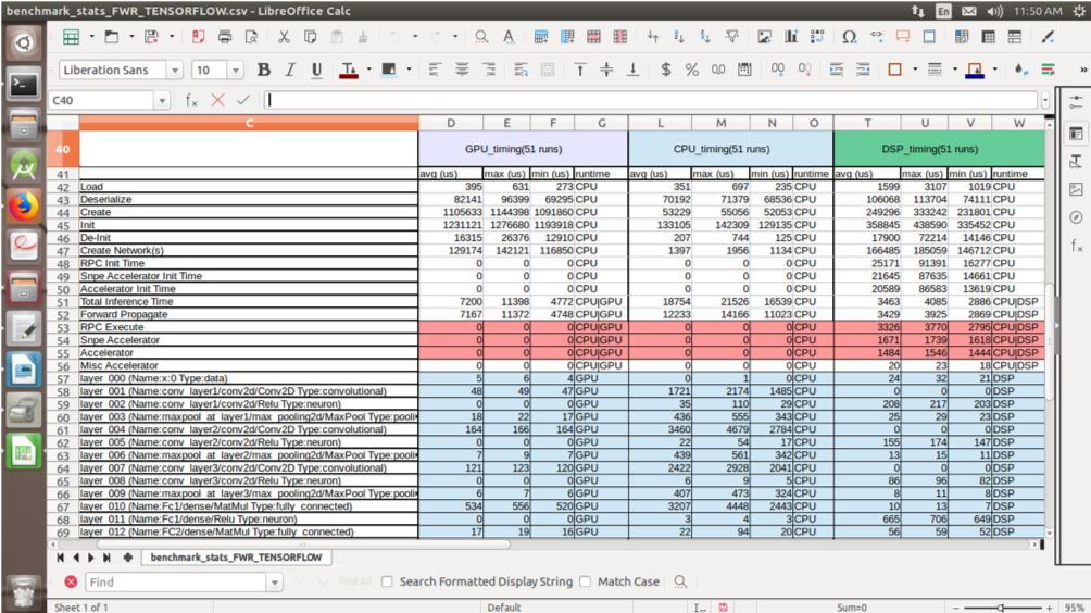
When pulled into a spreadsheet application and formatted — including cells and ranges colored for clarity — the output resembles the screenshot below.

Interpreting the results of snpe_bench.py

1. The excerpt below (cropped for clarity) shows the columns for execution on two runtimes: GPU_ub_float and CPU. The red-shaded figures show the actual inference time of the model, not including any time consumed for tasks such as loading the data, calling the API and waiting for a resource.

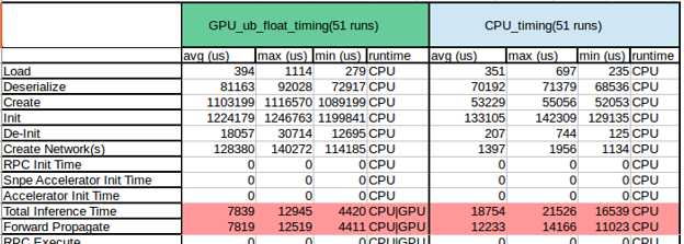
Total Inference Time is the total amount of time in microseconds from the entry point of snpe->execute() until it returns.

Forward Propagate Time is the amount of time that an individual runtime (CPU/GPU/DSP) takes to run the inference.

2. In the excerpt below, the blue-shaded figures show the actual inference made using the requested runtime.

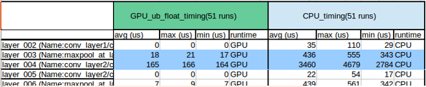
In the configuration file, setting CpuFallback to true ensures that, by default, any layers not supported by the respective runtime will be executed on the CPU. However, setting it to true is not recommended, because the main objective is to determine the inference time of each layer with different runtimes.

3. Note that it is not always the case that the higher processing power of the DSP compared to the GPU will result in higher performance of a model. The benchmarking report below shows the results of executing on GPU, CPU and DSP a facial expression recognition (FER) model built using Keras and converted to DLC format.

In the excerpt below (cropped for clarity), compare the average Total Inference Time for GPU to that for DSP.

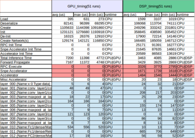
At first glance, the red-shaded figures suggest that the model runs much faster with the DSP runtime (3463 µs) than with the GPU runtime (7200 µs). But it is also necessary to account for the time consumed by RPC Execute (acts as a communicator between CPU, GPU and DSP), Snpe Accelerator and Accelerator. Those operations amount to 6481 µs on DSP and 0 µs on GPU.

For a low number of predictions, therefore, the FER model performs better on GPU than on DSP. If the application calls for a high number of predictions that will offset the overhead, then it will be worth running the model on DSP.

4. The blue-shaded figures show the individual processing time of each layer on different runtimes. Engineers can replace poorly performing layers with similarly functioning ones that consume less time.

5. The configuration structure for snpe_bench.py includes a Measurements parameter whose possible values are timing and mem. When set to mem, the output includes details of memory utilization by the model. The image below shows the sample memory report (modified here for clarity) of an individual iteration of an FER model.

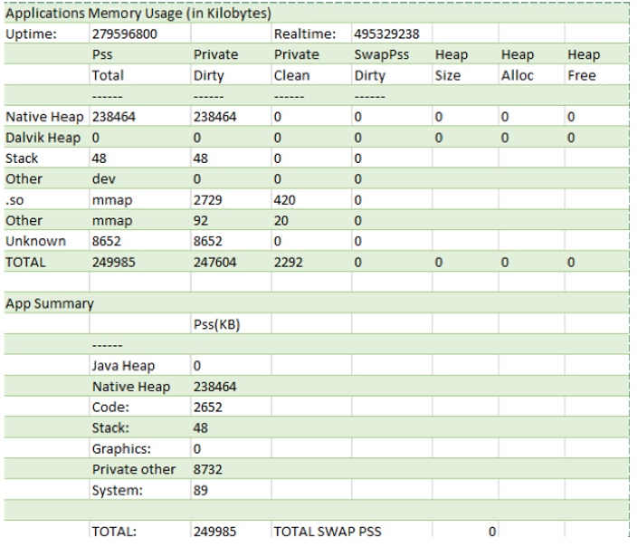
A summary report is also created using the individual memory report and can be seen in the results folder after completing the execution.

snpe-diagview

snpe-diagview generates a report of each iteration — timing information for each layer, and the entire forward propagate time — for analysis. The following command generates the report:

Qualcomm Neural Processing SDK is a product of Qualcomm Technologies, Inc. and/or its subsidiaries.