Advanced Computer Vision CNN Architectures
Visualization in GoogleNet Inception and ResNet
Visualization helps in exploring the layers responsible for extracting a specific feature. In the process of building a CNN model, visualizing layers is as important as calculating the training error (accuracy) and validation error. It also helps in using the pre-trained models for transfer learning, by visualizing and embedding only the required filters with specified weights for the current requirement. Visualization can be applied to heatmaps of class activation, filters and activation functions.
GoogleNet Inception
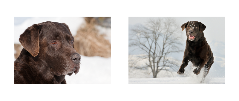
In GoogleNet Inception, multiple size filters are applied at the same level along with 1×1 convolution. It is not always possible to use the same filter to detect the object from an image. When running object detection and feature extraction on the images below, for example, it would be necessary to use a larger filter for the image on the left (close-up of brown dog) and a smaller filter on the image on the right (dog with tree in background).
(For a diagram of the architecture of GoogleNet Inception, see https://web.cs.hacettepe.edu.tr/~aykut/classes/spring2016/bil722/slides/w04-GoogLeNet.pdf, pp. 31-32.)
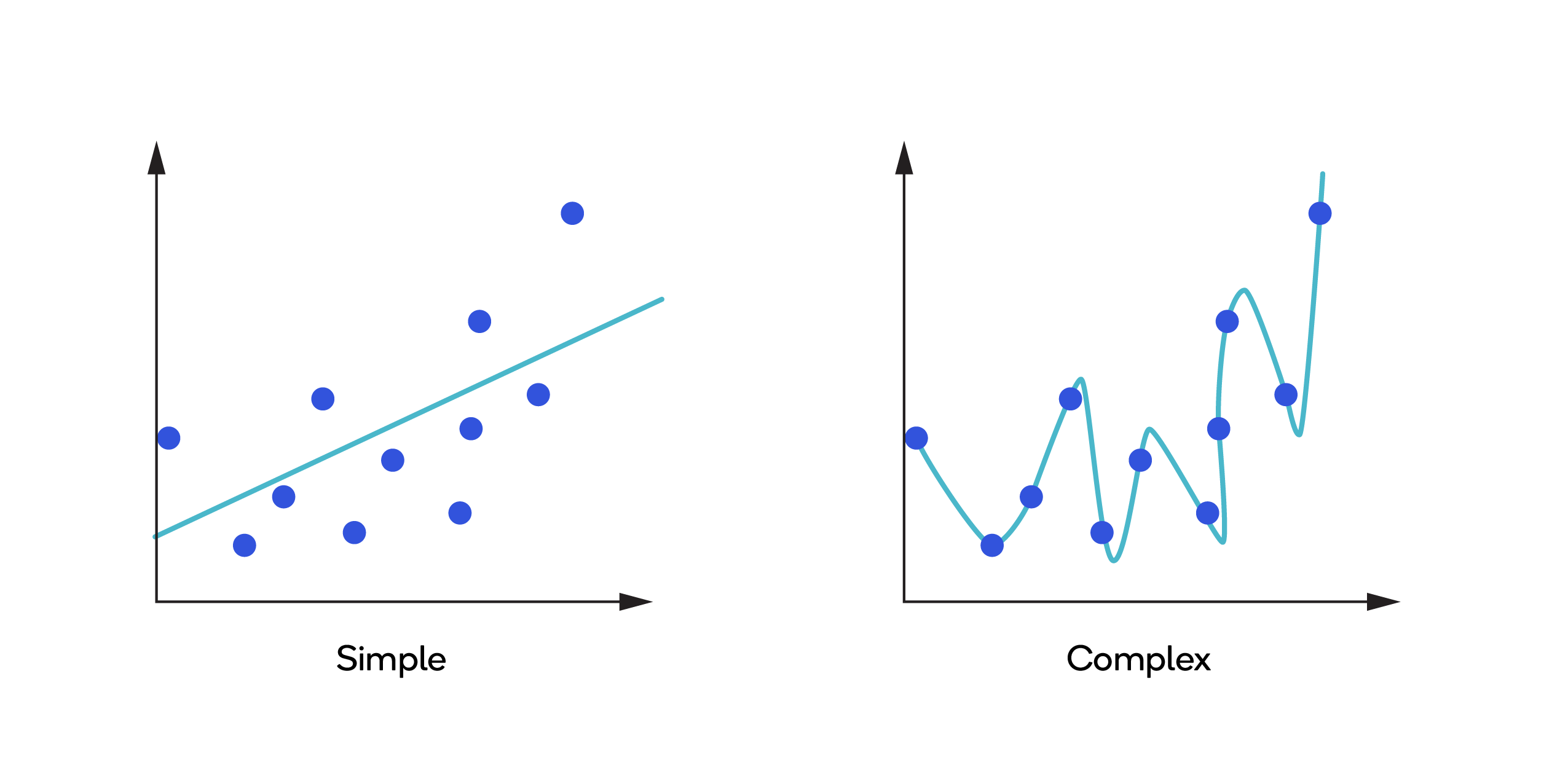
GoogleNet Inception helps in avoiding overfitting by increasing the width of the model relative to its depth. As the depth of the model increases to capture more features, the activation function is responsible for keeping the model from being too general due to overfitting the training data.
The images below depict general (simple) and overfitted (complex) models.
In GoogleNet Inception, filters with different sizes are applied to a single input because, as mentioned in the dog example above, object detection by feature extraction varies. Using filters of multiple sizes at the same level ensures that the objects of different sizes in different images are easily detected.
Before applying the filters, the input is convolved with a 1×1 matrix, reducing the number of computations made on the image. For example, an input of size 14×14×480 convolving with a filter of size 5×5×48 results in (14×14×48)×(5×5×480) = 112.9 million computations. But if the image is convolved with 1×1 before convolving with 3×3, the number of computations drops to (14×14×16)×(1×1×480) = 1.5 million and (14×14×48)×(5×5×16) = 3.8 million. A filter concatenation is used to collect all the filters of that inception block.
An inception block can also have an auxiliary branch. The auxiliary branches are present in the training-time architecture but not in the test-time architecture. They introduce more aggressiveness during classification when they encourage discrimination in the lower stages of the classifier. They increase the gradient signal that gets propagated back and they provide additional regularization.
ResNet
If the neural network is too deep, the gradient from the loss function will progress towards zero, a problem known as “vanishing gradient.” ResNet is used to solve this problem by skipping the connections backward from the later layers to the initial layers.
ResNet (Residual Network) contains four residual blocks: Layer1, Layer2, Layer3 and Layer4. (For a diagram of the architecture of ResNet, see https://towardsdatascience.com/understanding-and-visualizing-resnets-442284831be8.)
Each block contains a different number of residual units that perform a set of convolutions in a unique approach. Each block is augmented by max pooling to reduce the spatial dimensions.
As illustrated below, there are two types of residual units: baseline residual units and bottleneck residual units.
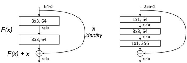
Baseline residual unit Bottleneck residual unit
The baseline residual unit contains two 3×3 convolutions with batch normalization and ReLU activations.
The bottleneck residual unit consists of three stacked operations with a series of 1×1, 3×3 and 1×1 convolution operations. The two 1×1 operations are designed for reducing and restoring dimensions. The 3×3 convolution is used to operate on a less-dense feature vector. Also, batch normalization is applied after each convolution and before ReLU non-linearity.