Snapdragon and Qualcomm branded products are products of
Qualcomm Technologies, Inc. and/or its subsidiaries.
Co-written with Hongqiang Wang and Alex Bourd
Our previous post about OpenCL optimization on the Qualcomm® Adreno™ GPU described several candidate use cases. In this post we’ll cover a two-step optimization for apps that use the Sobel filter. The optimization is based on data load improvement, OpenCL functions, and support for those functions in the Adreno GPU hardware.
Introduction to the Sobel filter
The Sobel filter is used in many image processing and computer vision algorithms for edge detection. It comprises two 3x3 kernels that compute the image derivatives in horizontal (X) and vertical (Y) directions. Figure 1 shows the two kernels.
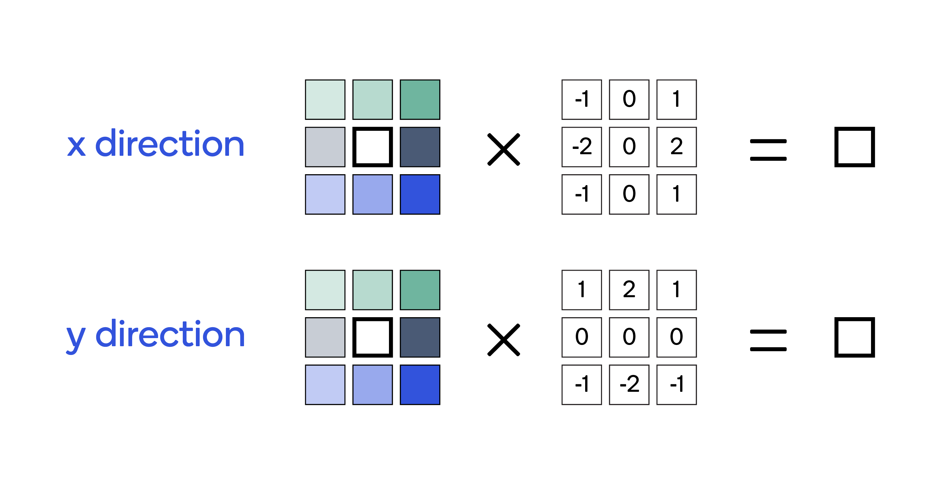 Figure 1: The two kernels for horizontal and vertical directions
Like other image processing operations, the Sobel filter is an embarrassingly parallel operation that is ripe for accelerating on a GPU. In this blog, we show how to use the GPGPU capabilities of the Adreno GPU to perform blazing-fast edge detection with this filter.
Naïve implementation
A naïve implementation is to have one work-item generate one filtered output pixel. To do this, each work-item needs to load 3x3 pixels; i.e., the center pixel corresponding to its global work-item ID, plus the neighboring 8 pixels. Assuming the input is a 2-dimensional, grayscale image with size of WxH, where W is width and H is height, the kernel needs to launch (WxH) work-items in total. Since each output pixel can be evaluated independently of other pixels, we have exploited the data-parallel nature of the problem.
So, what makes this approach naïve?
In a bid to parallelize arithmetic operations, we have neglected the efficiency of memory load operations and data reuse. Each input image pixel is loaded by 9 separate work-items; in other words, each work-item loads 9 pixels from the global memory, and that global memory is used only once by the work-item. This leads to unnecessary data traffic between global memory and the GPU cache, as well as between the GPU cache and ALU unit in the GPU. Therefore, the implementation makes the algorithm heavily memory-bound. Note that excessive memory traffic not only hurts performance, but more important, it also leads to significantly high power and energy consumption, the bane of mobile use cases.
In this naïve implementation, processing a 2D, grayscale image (3264x2448 pixels, 8-bit/pixel) on the Snapdragon™ 845 (Adreno 630) Mobile Hardware Development Kit would require 7.6 milliseconds (ms). Note that the number may vary, depending on several factors, such as the compiler and driver versions, and the clock rate (different vendors may choose slightly different clock rates for the GPU and CPU) of the device you are running with.
Our objective, then, is to ease this memory bottleneck by optimizing how we load pixels and reuse the data.
Open CL optimizations to accelerate the Sobel filter
To reduce the memory bottleneck, we use two optimization steps.
1. Data pack optimization
First, we make a change to improve the efficiency of data reuse. While the change is not specific to OpenCL or to the Adreno GPU, it is nevertheless an important step.
We recognize that each pixel can potentially be reused 9 times for the computation of 9 different outputs. Loading it every time from the global memory is the primary reason for the memory bottleneck. Instead, we could load the pixel into the register of a work-item and then reuse it for computing multiple outputs. This means that each work-item would compute MxN output pixels (each for horizontal and vertical kernels). To do this, it would load (M+2)x(N+2) pixels as in Figure 2.
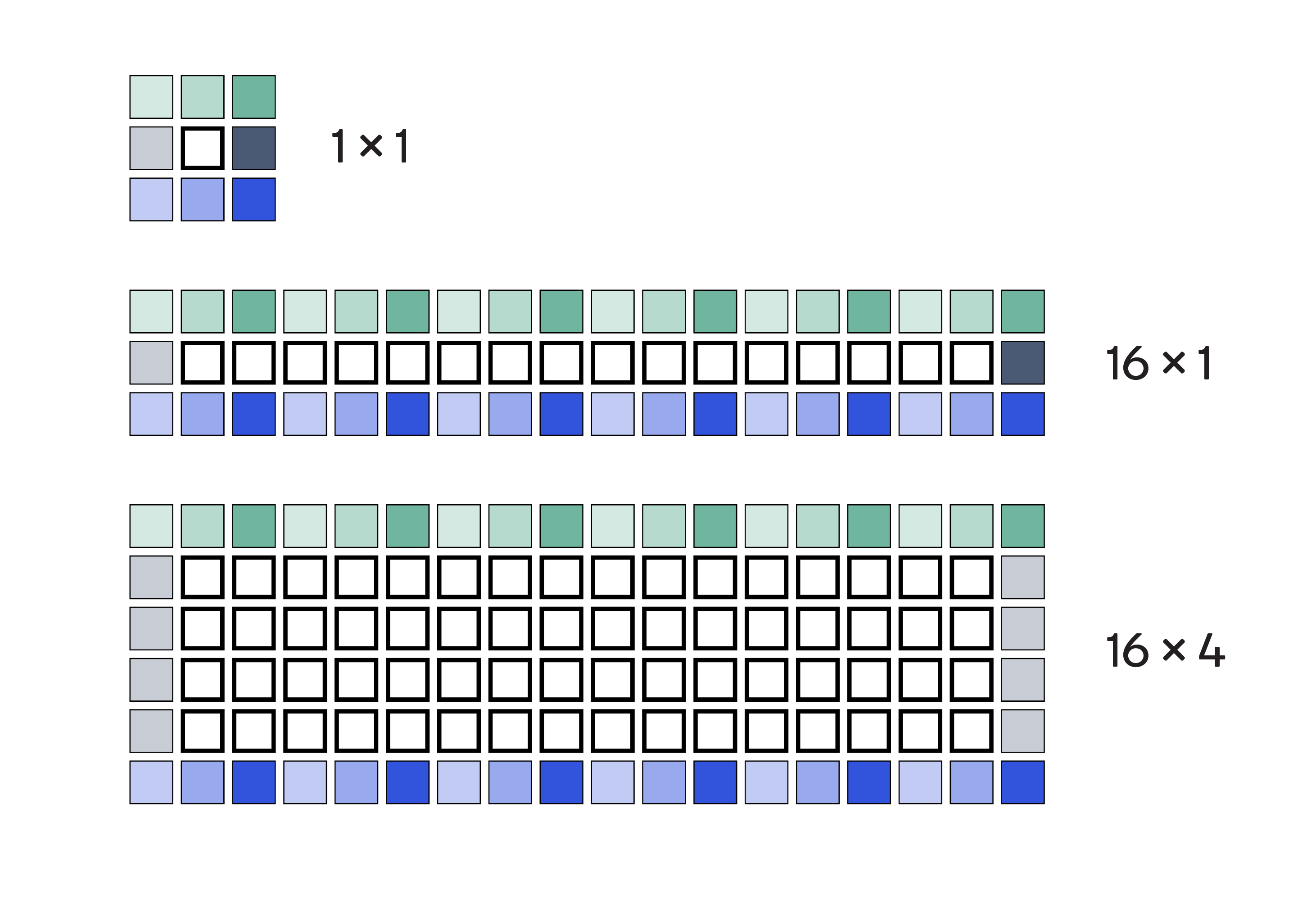 Figure 2: Load (M+2)x(N+2) pixels to compute MxN output pixels
Table 1 shows how, even as M and N increase (header row), the average number of input bytes for each output computation (row 3) decreases
| One pixel/work-item (naïve) | 16x1 pixel/work-item | 16x4 pixel/work-item | |
|---|---|---|---|
| Input bytes per work-item | 9 | 54 | 108 |
| Output bytes per work-item | 1 | 16 | 64 |
| Required input bytes per output | 9 | 3.375 | 1.68 |
Table 1: Average memory operations per output for varying M and N
The obvious question then is: How large should M and N be? Surely, we cannot load too much data for a single work item, because that would result in a higher register footprint and thus smaller workgroup size. At worst, this might cause register spilling, which would significantly impair performance.
We try 16x1 and 16x4 configurations of MxN to see the performance gains, choosing M=16 for vectorized reads of 128-bit chunks of data. This in fact is our next optimization step.
2. Vectorized load/store optimization
This step takes advantage of OpenCL functions and of the Adreno hardware that directly supports those functions.
The number of load/store operations can be further reduced by using the vectorized load/store functions in OpenCL. In general, we recommend for Adreno GPU that for each work item, data should be loaded/stored in chunks of multiple bytes (e.g., 64-bit/128-bit) to achieve better bandwidth utilization.
Also, we recommend using vectorized load/store instructions that take up to 4 components, e.g., vload4/vstore4. That is because, for vectorized load/store of more than 4 elements, e.g., vload8/vstore8, hardware has to split into multiple load/store instructions, which reduces efficiency.
With these considerations, we can load each 18-pixel line in two lines of OpenCL code as follows:
short16 line_a = convert_short16(as_uchar16(*((__global uint4*)(inputImage + offset))));short2 line_b = convert_short2(as_uchar2(*((__global uint2*)(inputImage + offset))));Note that after dereferencing, we typecast the data to short data type. That is because the Adreno GPU has twice the ALU computing capacity (measured in gflops) of a 16-bit data type, such as short and half-precision floating-point (also known as fp16), as compared to a 32-bit data type. In a case like this, where there is no precision loss, a 16-bit, short data type is preferable.
Table 2 shows how increasing M and N reduces the average number of load/store operations per output.
| 16x1 Vectorized | 16x4 Vectorized | |
|---|---|---|
| vloads per output | 6/16 = 0.375 | 12/64 = 0.187 |
| vstores per output | 2/16 = 0.125 | 8/64 = 0.125 |
Table 2: Average loads and stores after vectorization
Optimizations result in performance improvement: From 7.6 ms down to 2.9 ms
We apply the three kernels from Figure 2 (1x1, 16x1, 16x4) to a 3264x2448 sized image. As shown in Figure 3, the performance improves significantly with our optimizations (taller bars are better). Note that we have normalized the performance of 1x1, the naïve implementation, on the Snapdragon® 820 (Adreno 530) to 1.0, and graphed the other results relative to it.
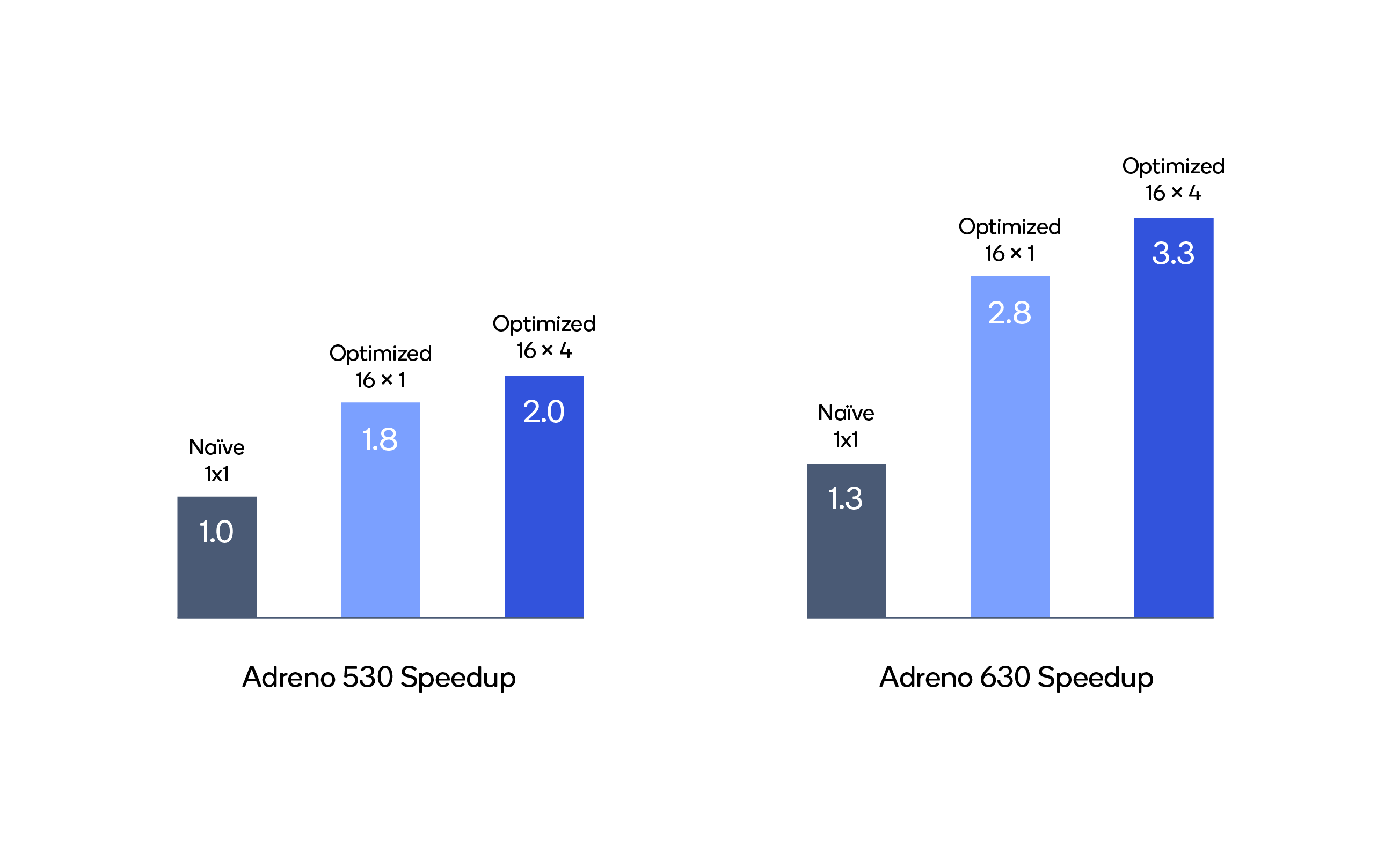 Figure 3: Results of the optimized kernels on Adreno 530 and Adreno 630
Translating those relative results into absolute numbers, it takes only 2.9 ms for the Adreno 630 to process a 3264x2448 sized, grayscale image — far less than the 7.6 ms before optimization.
Summary
In summary, we used three main ideas to optimize the Sobel filter and alleviate the memory bottleneck:
- Data packing improves the efficiency of data reuse.
- Vectorized load/store is the key to reducing the number of load/store operations.
- Short data type is preferred over integer or char type in this case.
Notably absent from this list is the use of local memory. This is deliberate because the data pack and vectorized load techniques used here have significantly improved the efficiency of data reuse and reduced memory traffic. Adreno GPUs typically have on-board, physical, local memory that has very short access latency from ALU; however, the use of local memory does not necessarily improve performance, largely due to the overhead associated with its usage. For example, a barrier is often required for data synchronization, thanks to the relaxed memory consistency model in OpenCL. In future blog posts we will elaborate on how to wisely use local memory for Adreno GPUs.
Apart from this, we could also use image instead of buffer object to take advantage of the built-in, hardware-accelerated texture engine and L1 cache in Adreno GPUs. We will introduce these techniques in a separate article on accelerating the Epsilon filter.
Next steps
If GPU programming is on your radar, then keep an eye out for upcoming blog posts as we continue exploring OpenCL optimization.
Meanwhile, have a look through the Snapdragon® Mobile Platform OpenCL General Programming and Optimization Guide for more ideas, and download the Adreno GPU SDK to see how you can accelerate your own algorithms.
Do you have an OpenCL optimization you’d like to see? Send me questions in the comments below or through the Adreno GPU SDK support forum.
Comments
Re: OpenCL Optimization: Accelerating the Sobel Filter on...
Re: OpenCL Optimization: Accelerating the Sobel Filter on...