Training, Testing and Evaluating Machine Learning Models
Training, evaluation, testing and accuracy
Model training
Model training for deep learning includes splitting the dataset, tuning hyperparameters and performing batch normalization.
Splitting the dataset
The data collected for training needs to be split into three different sets: training, validation and test.
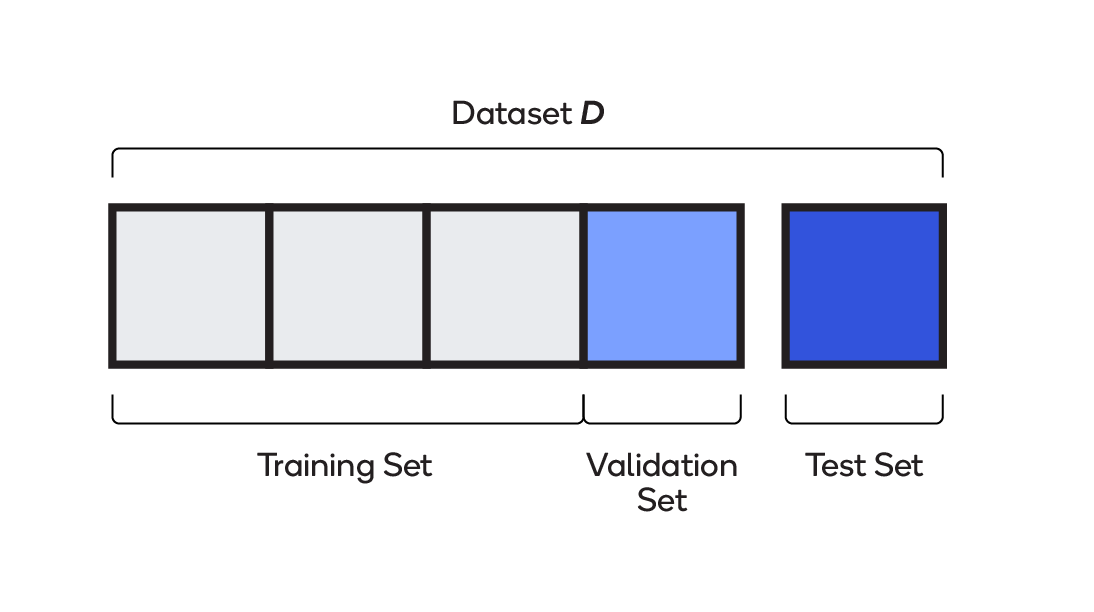
- Training — Up to 75 percent of the total dataset is used for training. The model learns on the training set; in other words, the set is used to assign the weights and biases that go into the model.
- Validation — Between 15 and 20 percent of the data is used while the model is being trained, for evaluating initial accuracy, seeing how the model learns and fine-tuning hyperparameters. The model sees validation data but does not use it to learn weights and biases.
- Test — Between five and 10 percent of the data is used for final evaluation. Having never seen this dataset, the model is free of any of its bias.
Hyperparameter tuning
Hyperparameters can be imagined as settings for controlling the behavior of a training algorithm, as shown below.
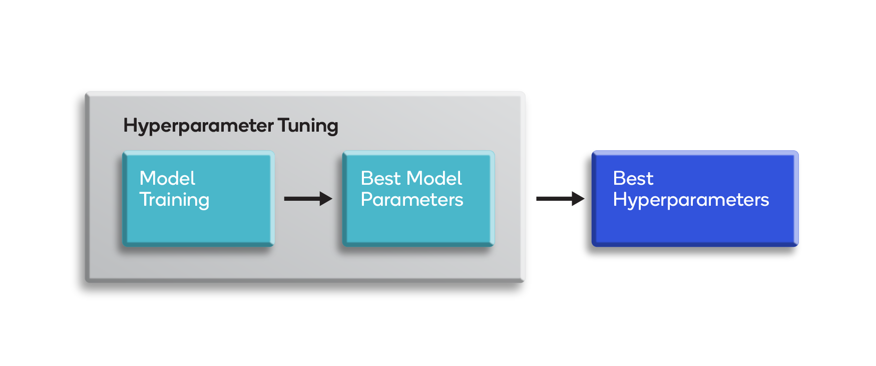
Based on human-adjustable hyperparameters, the algorithm learns parameters from the data during the training phase. They are set by the designer after theoretical deductions or adjusted automatically.
In the context of deep learning, examples of hyperparameters are:
- Learning rate
- Number of hidden units
- Convolution kernel width
- Regularization techniques
There are two common approaches to tuning hyperparameters, as depicted in the diagram below.
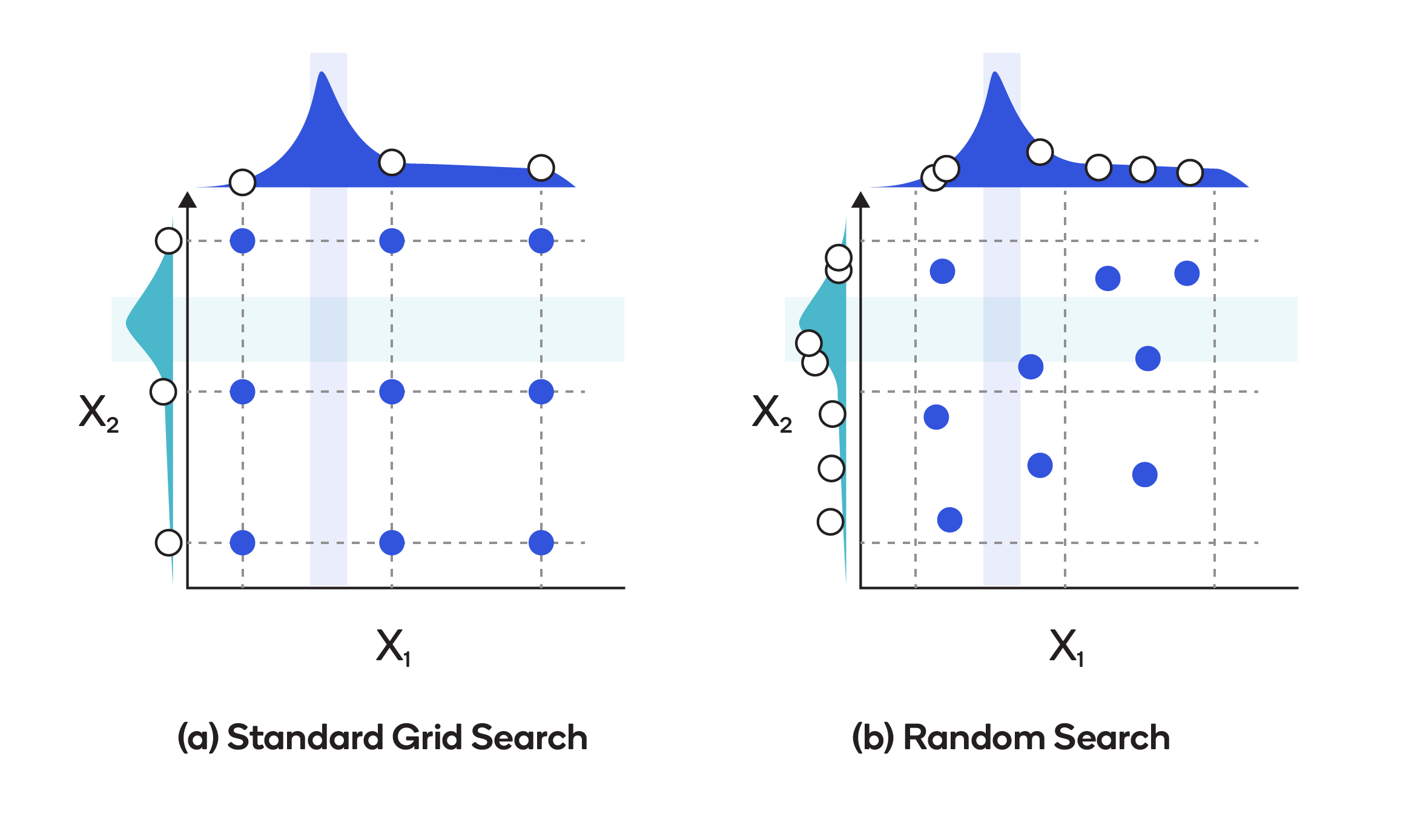
The first, standard grid search optimization, is a brute-force approach through a predetermined list of combinations of hyperparameters. All possible values of hyperparameters are listed and looped through in an iterative fashion to obtain the best values. Grid search optimization takes relatively little time to program and works well if the dimensionality in the feature-vector is low. But as the number of dimensions increases, tuning takes longer and longer.
The other common approach, random search optimization, involves randomly sampling values instead of exhaustively searching through every combination of hyperparameters. Generally, it produces better results in less time than grid search optimization.
Batch normalization
Two techniques, normalization and standardization, both have the objective of transforming the data by putting all the data points on the same scale in preparation for training.
The normalization process usually consists of scaling the numerical data down to a scale from zero to one. Standardization, on the other hand, usually consists of subtracting the mean of the dataset from each data point and then dividing the difference by the standard deviation of the datasets. That forces the standardized data to take on a mean of zero and a standard deviation of one. Standardization is often referred to as normalization; both boil down to putting data on some known or standard scale.
Model evaluation and testing
Once a model has been trained, performance is gauged according to a confusion matrix and precision/accuracy metrics.
Confusion matrix
A confusion matrix describes the performance of a classifier model, as in the 2x2 matrix depicted below.
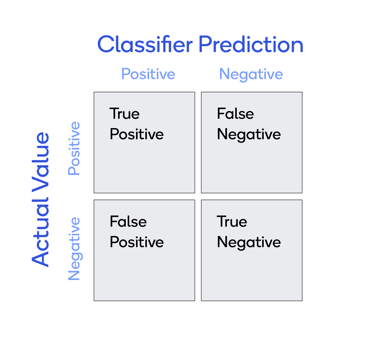
Consider a simple classifier that predicts whether a patient has cancer or not. There are four possible results:
- True positives (TP) — Prediction was yes and the patient does have cancer.
- True negatives (TN) — Prediction was no and the patient does not have cancer.
- False positives (FP) — Prediction was yes, but the patient does not have cancer (also known as a "Type I error").
- False negatives (FN) — Prediction was no, but the patient does have cancer (also known as a "Type II error")
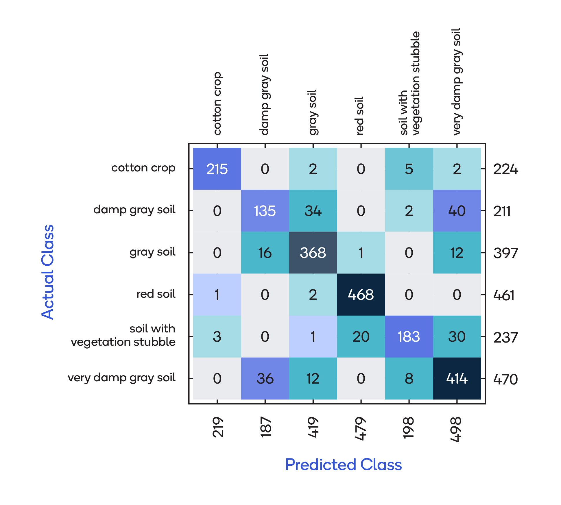
A confusion matrix can hold more than 2 classes per axis, as shown here:
Precision / Accuracy
It is also useful to calculate the precision and accuracy based on classifier prediction and actual value.
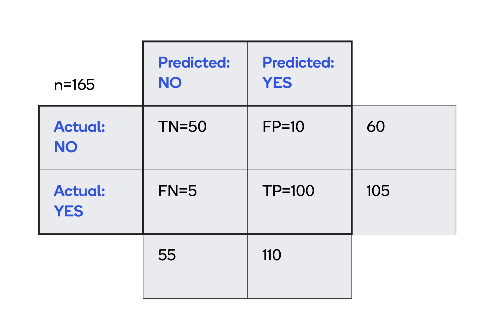
Accuracy is a measure of how often, over all observations, the classifier is correct. The calculation, based on the grid above, is (TP+TN)/total = (100+50)/(60+105) = 0.91.
Precision is a measure of how often the actual value is Yes when the prediction is Yes. In this case, that calculation is TP/predicted yes = 100/(100+10) = 0.91.